|
|
|
|
|
Filter Library Updated |
| We’ve
added about 1500 Laplace filters for Butterworth, Chebyshev, Bessel and
Elliptic transfer functions. For each of these methods there are 4 possible
types: Low Pass, High Pass, Band Pass and Band Stop. There are a variety
of pass-band ripple and attenuation values for different filter orders.
We output the coefficients with 15-digit precision. Computations are normalized
to 1 r/s so that computational accuracy is maintained for 10th order filters.
The Laplace model then scales its frequency so that designs in the GHz
region are well conditioned; that is, we don’t need to raise the actual
frequency to a high power that would result in numerical overflow. Figure
1 compares the performance of 3rd, 4th and 5th order low pass filters
that have been transformed into band pass filters using the following
formula:
We have made the software that generated these libraries
available to registered users on the web. Look on your SpiceNet “Help\Intusoft
Support\Paid Support.” This lets you fine tune filter specifications
and also get pole zero locations as well as Z transform coefficients.
Reasonable accuracy is achieved up to 10th order filters (note that order
doubles for band-pass/stop). |
|
|||||||||||||||||
|
|
||||||||||||||||||
Tips and Tricks |
|
To send a screen shot in an E-mail: use “<alt> + PrtScrn” to get the active window in the clipboard, then paste it into your email (using MS Word as your E-mail editor) Occasionally a SpiceNet drawing becomes corrupted so that Fit-To-Page no longer works correctly. It leaves the drawing pushed over to one side (or the top or bottom) of the screen. This usually happens because some component or label has gotten pushed outside of the visible portion of the drawing. (The cause has been fixed in Build 1900). In order for Fit-To-Page to work again, this object must be deleted. Just how do you do that if you can’t see it? The solution is to select “Drawing Page Size” from the Options menu. When the dialog is displayed, change the page size to “E (34x44)” and click “OK”. The offending object should then be visible. Delete it, or move it back to the main part of the drawing, and then change the page size back to the original value. Finally, don’t forget to save the change, so the problem will be gone next time you open the drawing. |
New !User Scripts |
|
Here are several scripts we have found useful in creating this newsletter: familyEYE.scp familyEye.scp is used to collapse a transient simulation into a family for viewing “eye” diagrams. Frequently “eye” diagrams are displaced in time using the familyEye script. Two user entries are used to setup the “eye” diagram. The numsteps variable is the number of plots in the “eye.” For example, if you run for 250 clock cycles, enter 250 for numsteps. The “shift” parameter is used to rotate the linearized waveform to the right to account for delays caused by filters or signal propagation. The waveform is linearized to have 4096 points, shift is the number of these points to rotate the waveform. You may want to play around with the shift value to align the “eye” properly. For very long waveforms, you may want to increase the linearize argument. The algorithm for the basic eye diagram is in http://www.intusoft.com/nlhtm/nl65.htm#sweeps. |
|
|
With the release of 8.x.10, Build 1843, the shift and arrow keys are available for hot key assignment. We used the up and down arrows to pan the y-axis and shift+up/down arrows to increase/decrease the scaling. Below are scripts that use the shift+left/right arrows to pan in the x axis. We couldn’t use the left-right arrows because they are used to move cursor1 along the waveform. The arrows are opposite the actual pan direction so that the waveform moves in the direction of the arrows, opposite to the direction of the viewing window. |
|
|
|
|
New ICL Commands |
|
|
| Format: assertvalid
<vecName> [<vecName>] ... Example: assertvalid vin vout All listed vector names are evaluated to insure that they represent either existing vectors, or vectors which are available from the Add Waveforms dialog. If any vector is not found, an error message is posted, and the script is halted. |
New Scope5 IEC EMI Scripts |
Check the web http://www.intusoft.com/in/Scripts/EMI
IEC SPECS/EMI IEC specs.html for new IEC 61000 Electromagnetic
Interference Specification Scripts for Class A, B, C, and D Equipment.
These specs describe harmonic current emission limits for household appliances
(Class A); portable tools and arc welding equipment (Class B); lighting
(Class C); and personal computers, televisions and monitors under 600W
(Class D). A format, example, and script for each equipment class is provided
on the web site. |
Costas Simulation |
|
Voltage Controlled Oscillator |
|
The code model sine wave generator can be used as a VCO;
however, the Costas VCO requires both sine and cosine signals to implement
quadrature detection. Instead of making a new code model, let’s see what
we can do with the existing models. The signals can be generated using
the sin( Then frequency becomes:
Where: FC is the carrier frequency |
|
|
|
Figure 2. VCO model with waveforms shows response to a frequency change of 50 meg rad/sec. |
|
Figure 2 shows the complete model. The Laplace code model was selected so that a true integrator is used, having infinite gain at DC. The input function, B3, is set to 0 initially. The integrator output is also initialized to 0 by setting the out_ic parameter to 0. Simulation using the code model sine wave generator runs about twice as fast; however, it has no cosine output or provision for initial phase error. The VCO model was wrapped into a subcircuit, VCO2phase, and stored as a behavioral function block. We’ll come back to this model after discussing the remaining behavioral components. Generating
a Test Signal Tapped shift registers with feedback are frequently used to generate pseudo random binary patterns, one such arrangement is shown in Figure 3. The exclusive or function is performed using selected shift register taps. It turns out that certain combinations will produce a data sequence that contains 2n-1 data patterns, where n is the length of the shift register. These patterns are sufficiently random to be useful for spread spectrum communications. For our test purpose, we can just use the code produced by the shift register to generate the modulation signal. The filter is scaled for a 10GHz clock. We’ll rescale it for a 10MegHz data clock and use a 900MegHz carrier. The signal can be captured using Scope5 and made into a PWL source for IsSpice. The Scope5 data accuracy must be set high enough to resolve the time axis so that each x axis value is unique. Eight digits will do the trick. Fewer digits may produce successive x-axis values that are the same resulting in a IsSpice run time error. The PWL table will be created in the output record and it can be pasted into a Spice voltage source, PWL generator. Next, it’s a matter of putting the pieces together. The phase detectors are simple behavioral multipliers. We have 3 choices for data filters:
Figure 3. Shift register generates pseudo random noise. See page http://www.intusoft.com/support.htm to find out how to get many more filter choices. There is no filter about the carrier since our test circuit modulator shaped the input spectrum. You can add noise or other interfering signals to the test signal and insert the carrier filter to evaluate its effect. The loop shaping filters, LPF1/2, have their bandwidth set by parameter WFIL1. The noise filter bandwidth, LPF3, is set to 10*WFIL1. KVCO is set to 8*WFIL1/(2*pi) in accordance with [Reference 1]. The complete Costas loop simulation is shown in Figure 4.
Figure 4. The complete Costas loop simulation. The “eye” diagrams for the Bessel filter and the LC filter are shown in Figure 5. As the filters become more of a brick wall, the constant delay feature gives way to a ringing response creating inter-symbol cross talk that tends to close the eye, reducing noise margin. For Bessel filters, W*T = sqrt(2*n-1)*ln(2) - .788/(6.5+n). Bessel function “bandwidth” is typically specified as 1/T, requiring adjustment for W, the actual bandwidth (2*pi*F). For a 5th order filter, 2*pi*Fc*T = 2.01 and 1/T = 2*pi*Fc/2.01
The equation has been evaluated in Table 1. You can have both phase and frequency offsets as well as noise added to the signal to evaluate lock time. It is interesting to note that for the case of a frequency offset, Vcntrl, in Figure 4 must have a corresponding DC value to remove the offset when the loop is locked. That offset will produce noise that appears to be random (because the data pattern is random and it is multiplied by the offset in the X4 mixer) that will throw the loop out of lock for high frequency offsets. |
|
Table 1.
|
|
|
Bessel 1 Filter Bandwidth Varies with Filter Order
|
|
| W*T | n |
| 1.10786 | 2 |
| 1.46698 | 3 |
| 1.75885 | 4 |
| 2.01092 | 5 |
| 2.23587 | 6 |
| 2.44081 | 7 |
| 2.6302 | 8 |
|
References [1] Jeff Feigin Practical Costas Loop Design, RF Design, Jan 2002, pg. 20 [2] D. Gollman and W.G. Chambers. Clock-controlled shift registers: A Review. IEEE Journal on Selected Areas in Communications (4) 7 (1989), pgs.525-533. |
FFT, Leakage and Filters |
|
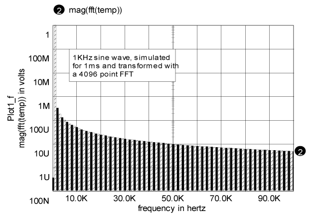
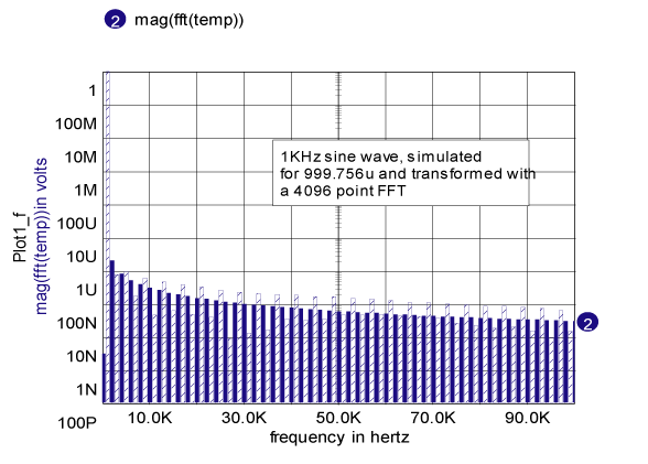
The Fast Fourier Transform, FFT, implements a computer algorithm that performs an N point Discrete Fourier transform, DFT, in a time that increases proportional to N*Log(N), which is considerably faster than the brute force approach that increases computational time as N squared. The DFT produces a Fourier series that has been truncated at N points. In doing this, the frequency domain view is representing a time domain signal that is periodic about the N points. When the time data is constructed, the value of the first point must be the same as the value of the N+1 point. It is a common error to make the first point and the last point of an IsSpice simulation identical. In the world of Fourier Transforms, that results in 2 successive time points with the same value. That causes what is commonly called leakage, the production of high frequency spectral artifacts (see Figure 6). As you increase the number of points in the FFT, these artifacts are diminished. If your simulation time is synchronous with simulation data, then you can avoid leakage by stopping the simulation 1 point before it begins to recur (see Figure 7). Ordinarily, the Scope5 FFT interpolates data into a FFT space that has N=4096 points in time. The number of points can be set anytime after a vector has been plotted, but before running any transforms. You need to stop the simulation at (N-1)/N*Tperiod to avoid leakage. For example, generate a sine wave at Freq, frequency and run the simulation from TSTEP to (N-1) /(N*Freq). For Freq = 1k and N=4096. |
|
 |
|
Figure 6. Leakage from mismatched simulation time
and period.
|
 |
|
Figure 7. Leakage removed by correct choice of simulation
period with respect to the FFT size.
|
So you can get a lot more accuracy in you transformed data if you: |
|
|
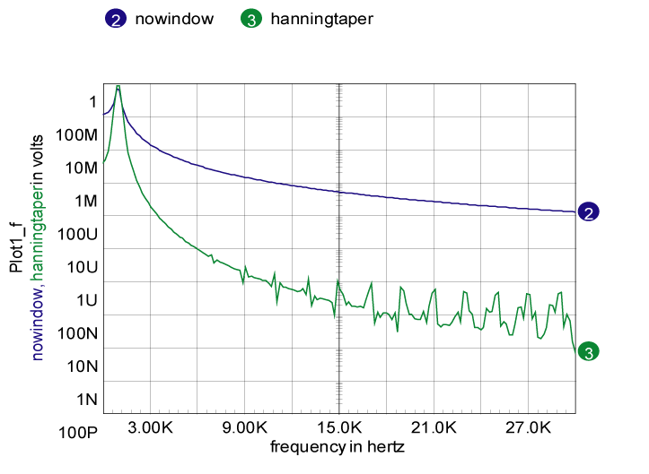
Probably the hardest to do is the third item. If you have oscillators that are running based on computed state variables, then the simulation period will be asynchronous with respect to the simulator time step. This problem is common to real hardware and the solution is to pass the signal through a window. The time series is multiplied by a window that is constructed to make the starting point and ending point converge on the same value. This will reduce the higher frequency artifacts at the expense of broadening the lower frequency spectrum. Commonly used windows are available in the Scope5 calculator/build menu. Figure 8 illustrates this using a 5.5 ms time simulation span with a 1kHz sine wave with and without a hanning window. There is considerable broadening of the 1KHz spectrum; however, the high frequency artifacts are down by about 60dB. |
 |
|
Figure 8. Waveform 3 has improved accuracy by applying
a cosine (Hanning) window.
|
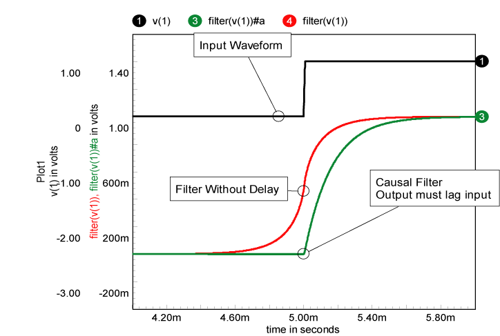
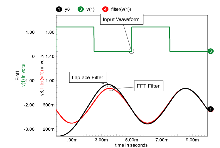
Besides using the FFT for spectral analysis, you
can make time domain filters. This is accomplished by transforming the
time series to a complex frequency series and multiplying by the conjugate
of the filter function, then transforming back to time domain. We have
added a number of conjugate filter functions to the ICL. These include
Bessel, Butterworth, Chebyshev and Elliptic functions. If you replace
the conjugate filter with its magnitude, the result is a cosine filter
( cos(re) + jsin(im) ® cos(mag) + j0). Since phase = atan(im/re) =
0, there is no phase shift and hence no time delay. These filters are
good for removing noise from historical data without temporal lag. Figure
9 compares these 2 filters. |
 |
|
Figure 9. Comparison of causal filter and filter
without delay.
|
|
|
 |
|
Figure 10. Comparison of filters during and after
simulation.
|